Timing of HD 332231
Here we will be using tracit to study HD 332231, while accounting for TTVs
Firstly we import tracit. The two run commands are just to setup text rendering in the plots to LaTeX.
[1]:
import tracit
We’ll create two structures:
For the parameters, priors, boundaries, etc.
For our data, and we can also specify the de-trending/noise model
We’ll call the first one ‘par’ and the second one ‘dat’.
[2]:
par = tracit.par_struct(n_planets=1,n_phot=1,n_spec=1)
dat = tracit.dat_struct(n_phot=1,n_rvs=1,n_ls=0,n_sl=0)
For the parameter structure we specified that we have 1 planet in the system, 1 photometric system, and 1 spectroscopic system (RVs, shadow, or slope).
For the data we also define the number of photometric systems, while we further specify the type of spectroscopic measurements\(-\)n_rvs for RVs, n_ls for the shadow (lineshape), or n_sl for the subplanetary velocity (slope).
We then specify the filenames, and that we want to fit the photometry, radial velocities with the inclusion of the RM effect.
[3]:
dat['RV filename_1'] = 'rv_HD332231.txt'
dat['LC filename_1'] = 'lc_HD332231.txt'
dat['Fit RV_1'] = 1
dat['RM RV_1'] = 1
dat['Fit LC_1'] = 1
Then we’ll initilize the data, i.e., load in the .txt files.
[4]:
tracit.ini_data(dat)
tracit.run_bus(par,dat)
Here we’ll load in a (good) result from a previous run, so we don’t have to set all the parameters. We first use pandas to load in the .csv file into a DataFrame, which we then pass on to the update_pars function along with our par structure to update it.
[5]:
import pandas as pd
rdf = pd.read_csv('results_from_old_fit.csv')
tracit.update_pars(rdf,par,best_fit=False)
Before we run our MCMC, it’s a good idea to check that our parameters/data look reasonable. We therefore plot the light curve and the radial velocity curve.
[6]:
pre_inspect = 1
if pre_inspect:
tracit.run_exp(1)
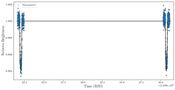
tracit.plot_lightcurve(par,dat)
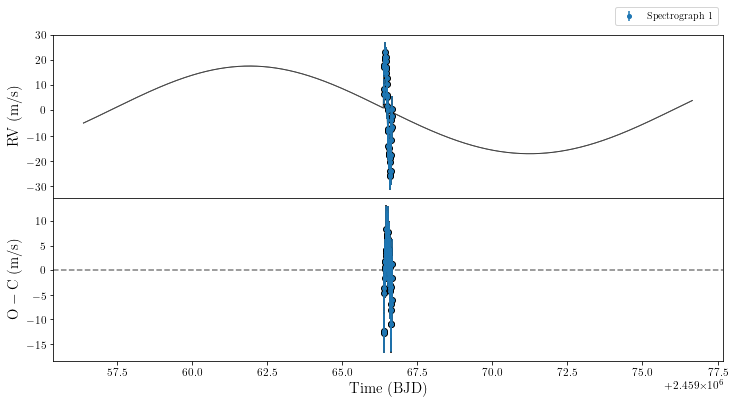
tracit.plot_orbit(par,dat)
## Photometric system 1/Photometer 1 ##:

Reduced chi-squared for the light curve is:
         0.695
Number of data points: 1200
Number of fitting parameters: 0
#########################
## Spectroscopic system 1/Spectrograph\ 1 ##:

Reduced chi-squared for the radial velocity curve is:
         13.617
Number of data points: 42
Number of fitting parameters: 0
#########################
/home/emil/anaconda3/lib/python3.7/site-packages/IPython/core/pylabtools.py:132: UserWarning: Creating legend with loc="best" can be slow with large amounts of data.
  fig.canvas.print_figure(bytes_io, **kw)
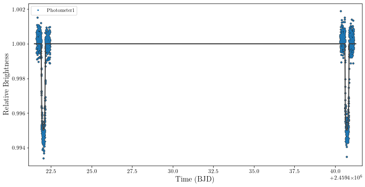
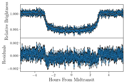
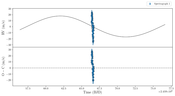
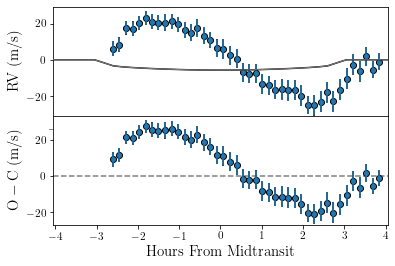
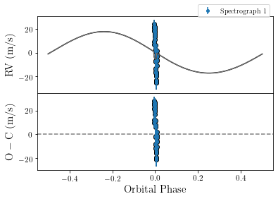
There’s obviously room for some improvement here. \(R_{\rm p}/R_\star\) seems to be too small, \(\lambda\) is close to \(90^\circ\), and what is perhaps less obvious is that while the timing, \(T_0\), for the transit in the TESS photometry is alright, there is a shift in timing for the HARPS-N data showing the RM effect. Let’s hope our MCMC can fix that.
We’ll first list the parameters we want to fit, and as we here have a bit of an unusual parameter, ‘Spec_1:T0_b’, we’ll run it through the check_fps function to create an entry for that parameter. ‘Spec_1:T0_b’ will let the mid-transit time for planet ‘b’ using the spectroscopic data from ‘1’ float freely (as freely as the prior applied, at least).
[7]:
par['FPs'] = ['T0_b','Rp_Rs_b','lam_b','Spec_1:T0_b']
tracit.check_fps(par)
Then we’ll specify the priors, and their boundaries (for the sake of convergence we’ll be a bit restrictive):
[8]:
par['lam_b']['Prior'] = 'uni'
par['lam_b']['Prior_vals'] = [0,2,-180,180]
par['Rp_Rs_b']['Prior'] = 'uni'
par['Rp_Rs_b']['Prior_vals'] = [0.069,0.001,0.05,0.1]
par['Spec_1:T0_b']['Prior'] = 'uni'
par['Spec_1:T0_b']['Prior_vals'] = [2458729.6819,0.05,2458729.6,2458729.8]
par['T0_b']['Prior'] = 'tgauss'
par['T0_b']['Prior_vals'] = [2458729.681,0.0005,2458729.6,2458729.8]
for the MCMC we can specify the number of CPUs we have at our disposal through nproc. We can also generate some instructive plots that allow us to inspect how the MCMC was performing; we can inspect how the walkers were walking using the chains argument, and we can see the 2D correlation plot through the corner argument.
We will do 10,000 draws with 20 walkers.
[9]:
mc = 1
if mc:
    ndraws = 5000
    nwalkers = 20
    nproc = 1
    ndf = tracit.mcmc(par,dat,ndraws,nwalkers,nproc=nproc,corner=True,chains=True)
Fitting T0_b.
Fitting Rp_Rs_b.
Fitting lam_b.
Fitting Spec_1:T0_b.
Fitting 4 parameters in total.

Maximum number of draws is 5000.
Starting from 0 draws.
5000 draws remaining.
50%|█████ | 2500/5000 [10:59<10:59, 3.79it/s]
MCMC converged after 2500 iterations.
Burn-in applied: 1250
Chains are thinned by: 7
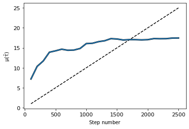
Even though we set the number of draws to 10,000, the routine stopped earlier because the MCMC had converged. After this we might want to take a look at the resulting parameters, which are both saved to ‘results.csv’, but also returned in the dataframe ndf.
Let’s print our new DataFrame with the results.
[10]:
print(rdf)
   Parameter                   P_b                    Spec_1:T0_b  \
0      Label  $P \rm _b \  (days)$  $T \rm _{0,b} \ (BJD) Spec_1$
1     Median              18.71205                    2458729.695
2      Lower              1.00E-05                          0.002
3      Upper              1.00E-05                          0.002
4   Best-fit             18.712051                    2458729.694
5       Mode              18.71205                    2458729.695
6      Prior                   uni                            uni
7   Location             18.712062                    2458729.681
8      Width               0.00023                       0.000275
9      Lower                18.703                     2458729.65
10     Upper                 18.72                     2458729.73
11      Rhat      1.00336135317264               1.00326246490288

                      T0_b                         Rp_Rs_b  \
0   $T \rm _{0,b} \ (BJD)$  $(R_\mathrm{p}/R_\star)\rm _b$
1             2458729.6814                           0.064
2                   0.0004                          0.0003
3                   0.0004                          0.0003
4             2458729.6819                          0.0694
5             2458729.6814                           0.069
6                      uni                             uni
7              2458729.681                         0.06976
8                 0.000275                            0.05
9               2458729.65                               0
10              2458729.73                             0.1
11        1.00429964195603                 1.0039305961874

                  a_Rs_b                 K_b                        lam_b  \
0   $(a/R_\star) \rm _b$  $K  \rm _b\ (m/s)$  $\lambda \rm _b \ (^\circ)$
1                   24.3                17.5                           90
2                    0.3                 1.2                           12
3                    0.4                 1.1                           12
4                   24.7                17.4                           11
5                   24.4                17.6                           -1
6                    uni                 uni                          uni
7                  24.21                17.3                            1
8                      1                 1.2                           10
9                     19                  10                         -180
10                    28                  30                          180
11      1.00399961064831    1.00353445827666             1.00321572158624

              cosi_b                     ecosw_b  ...                  inc_b  \
0    $\cos i \rm _b$  $\sqrt{e} \ \cos \omega_b$  ...  $i \rm _b \ (^\circ)$
1              0.006                        0.11  ...                  89.67
2              0.005                        0.09  ...                   0.15
3              0.003                        0.12  ...                   0.29
4              0.005                        0.12  ...                  89.71
5              0.004                        0.16  ...                  89.79
6                uni                         uni  ...                Derived
7               0.01                           0  ...                Derived
8               0.01                      0.0001  ...                Derived
9                  0                          -1  ...                Derived
10                 1                           1  ...                Derived
11  1.00532151468678            1.00366428157889  ...                Derived

           b_b                    T41_b                    T21_b  \
0   $b \rm _b$  $T \rm _{41,b} (hours)$  $T \rm _{21,b} (hours)$
1         0.14                    6.141                    0.404
2         0.12                    0.017                     0.01
3         0.06                    0.019                    0.008
4         0.13                    6.128                    0.404
5         0.14                    6.138                    0.397
6      Derived                  Derived                  Derived
7      Derived                  Derived                  Derived
8      Derived                  Derived                  Derived
9      Derived                  Derived                  Derived
10     Derived                  Derived                  Derived
11     Derived                  Derived                  Derived

              RV1_q1            RV1_q2            LC3_q1            LC3_q2  \
0   $q_1: \ \rm RV1$  $q_2: \ \rm RV1$  $q_1: \ \rm LC3$  $q_2: \ \rm LC3$
1               0.55              0.23             0.258             0.294
2               0.04              0.04             0.014             0.014
3               0.04              0.04             0.014             0.014
4               0.49              0.18             0.237             0.273
5               0.55              0.24             0.258             0.294
6            Derived           Derived           Derived           Derived
7            Derived           Derived           Derived           Derived
8            Derived           Derived           Derived           Derived
9            Derived           Derived           Derived           Derived
10           Derived           Derived           Derived           Derived
11           Derived           Derived           Derived           Derived

                  lnL      chi2
0   $\ln \mathcal{L}$  $\chi^2$
1              325059     1.022
2                   4     0.006
3                   4     0.006
4              325040     0.995
5              325059     1.022
6             Derived   Derived
7             Derived   Derived
8             Derived   Derived
9             Derived   Derived
10            Derived   Derived
11            Derived   Derived

[12 rows x 45 columns]
Finally, we probably want to see that things have actually improved. Therefore, we plot the data again, again we update our parameter dictionary with our new parameters before plotting.
[11]:
post_inspect = 1
if post_inspect:
    tracit.update_pars(rdf,par)
    tracit.plot_lightcurve(par,dat)
    tracit.plot_orbit(par,dat,updated_pars=rdf)
## Photometric system 1/Photometer 1 ##:

Reduced chi-squared for the light curve is:
         0.698
Number of data points: 1200
Number of fitting parameters: 4
#########################
## Spectroscopic system 1/Spectrograph\ 1 ##:

Reduced chi-squared for the radial velocity curve is:
         1.509
Number of data points: 42
Number of fitting parameters: 4
#########################
/home/emil/anaconda3/lib/python3.7/site-packages/IPython/core/pylabtools.py:132: UserWarning: Creating legend with loc="best" can be slow with large amounts of data.
  fig.canvas.print_figure(bytes_io, **kw)
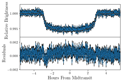
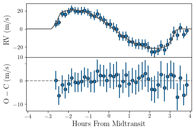
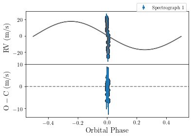
Arguably this looks much better.